Dirichlet Process Mixtures and Inference (Part 1)

Statistical inference often requires modeling the distribution of data. There are two branches of statistical modeling: parametric and non-parametric methods. The former one specifies the data distribution using a family of distributions with a finite number of parameters. In non-parametric methods, there is no limit on the number of parameters, which makes the name non-parametric a bit misleading.

One family of the non-parametric methods is well known and has been studied for a long time for its application in clustering: the Dirichlet Process Mixtures. Specifically, when you are dealing with a mixture model, the number of clusters is left as a hyper-parameter that requires tuning. However, in the Dirichlet Process Mixtures (DPM), we can also infer the number of clusters. Before we discuss the DPM, we will cover the Dirichlet Process (DP).

Dirichlet Process

In short, the Dirichlet Process is a generalization of Dirichlet distributions where a sample from the Dirichlet Process generates a Dirichlet distribution. Since its sample is a distribution, we also call it a distribution over distributions. Interestingly, the generalization allows the Dirichlet Process to have an infinite number of components (or clusters). For this, the DP is a non-parametric method, which means that there is no limit on the number of parameters. In practice, however, due to practical limitations on memory, computation, and time, we use the Truncated Dirichlet Process (TDP) during inference, which puts a limit on a number of clusters and therefore parameters. Also in real data, you will only get as many clusters as the number of data points :)

In this post, we will only consider the definition and one particular sampling procedure of the DP. We will cover the DPM and inference processes (inferring the number of clusters, as well as the parameters of the clusters) in the following posts.

Dirichlet Distribution

First, let the Dirichlet distribution with parameter $\mathbf{a} \in \mathbb{R}_{++}^K$ (K categories) be $Dir(\mathbf{a})$. If you haven’t picked up a probability book in years and you are fuzzy on the details, you only need to know that one of the properties of the Dirichlet distribution is that it is a conjugate prior of a multinomial distribution and thus has the following property. Let $A_k$ be the set of data from the $k$th category.

$$ \begin{align} P(\theta \in A) & \sim Dir(\mathbf{a}) \\ \boldsymbol{\theta} & = (\theta_1, ..., \theta_N) \quad N \text{ samples} \\ n_k & = |\{i : \theta_i \in A_k\}| \quad \text{number of samples in category } k \\ \mathbf{n} & = (n_1, ..., n_K) \\ P(\theta_{N+1} | \boldsymbol{\theta}) & \sim Dir(\mathbf{a} + \mathbf{n}) \end{align} $$

This is too much formality, but it will be helpful for the notation which I will use later. Basically, it says that if you observe $N$ samples and $n_k$ of them fall into the $k$th class, the posterior distribution after you observe the $N$ samples will be skewed to favor classes with more samples and the contribution is simply additive.

Definition of the Dirichlet Process

The formal definition of the Dirichlet Process is similar to that of many stochastic processes: the marginals of a distribution or a partition of a space follow a certain distribution. Here, as the name indicates, the partition of a space follows the Dirichlet distribution.

For example, let the space $A$ be a real number and a $K$-partition of the space is equivalent to making $K$ clusters in the space (this clustering effect gives us another way to generate samples by de Finetti’s theorem. I will not cover this in this post). If I denote the Dirichlet Process as $G$, then

\[(G(A_1), ..., G(A_K)) \sim Dir(a_1, ..., a_K)\]

Think of $G(A_i)$s as random variables that follow the Dirichlet distribution. More formally, let the base distribution be $H$ and the concentration parameter be $\alpha$.

\[(G(A_1), ..., G(A_K)) \sim Dir(\alpha H(A_1), ..., \alpha H(A_K))\]

For example, let $H\sim \mathcal{N}(0, 1)$ and $\alpha$ be an arbitrary positive number. In this case, since the base distribution is a Gaussian, we will sample from the Gaussian when we sample a new cluster. If we sample multiple distributions from the Dirichlet Process, the average of the whole process will be the Gaussian, i.e. $E[G(A)] = \mathcal{N}(0, 1)$. $\alpha$ also plays an interesting role. The variance of the Dirichlet process will be smaller as we choose a larger $\alpha$. If you are interested in more details, please refer to a great tutorial by Teh et al. 2010 ¹.

In light of all this, we can generate distributions from the Dirichlet process.

Samples from a Dirichlet Process

From the above definition, and from the conjugacy of the Dirichlet distribution, we can elicit a posterior distribution given $N$ observations $\boldsymbol{\theta}$.

$$ \begin{align} (G(A_1), ..., G(A_K)) | \boldsymbol{\theta} & \sim Dir(\alpha H(A_1) + n_1, ..., \alpha H(A_K) + n_K)\\ G | \boldsymbol{\theta} & \sim Dir((\alpha + N)H'(A_1), ..., (\alpha + N) H'(A_K)) \end{align} $$

where $H’ = \frac{1}{\alpha +N} \left(\alpha H + \sum_{i=1}^N \delta_{\theta_i}\right)$. The $\delta_{\theta_i}$ is a point mass on a sample $\theta_i$. In sum, the posterior distribution will be a new Dirichlet process with concentration parameter $\alpha + N$ and base distribution $H’$.

If we dissect the new base distribution, we can observe that

• With probability $\frac{\alpha}{\alpha + N}$, we sample from $H$.
• With probability $\frac{n_k}{\alpha + N}$, we sample from $A_k$.

Blackwell-MacQueen Urn Scheme

We know from above that the posterior distribution follows the base distribution $H$ with a certain probability or we otherwise sample from the existing pool. We can then generate a set of samples using the posterior distribution.

The sampling strategy that we just generated is called the Blackwell-MacQueen Urn scheme where the space $A$ is the space of color and we are drawing colored balls.

In the following SVG, I implemented a simple Blackwell-MacQueen Urn Scheme in javascript and d3.

I chose $\alpha = 5$ and a base distribution $H = \mathcal{N}(0, 1)$. To start, press the start button. It starts sampling each point. Since the base distribution follows the standard distribution, the expectation of all of the processes is 0 and thus we will be able to see most samples around 0. To see different samples from the Dirichlet Process, refresh the window and press start.

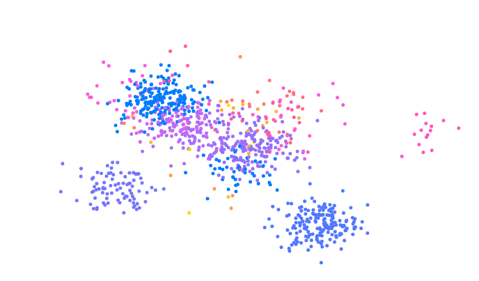
Another interesting property of the Dirichlet Process is the clustering effect. To see the clustering effect more closely, I visualized each cluster according to the cluster ID. If a new datum is sampled from a base distribution, not from the existing clusters, then it will be given a new cluster ID.

You will see few dominant ‘rich’ clusters getting ‘richer’ and taking up major portions of the data.

In the next post, I’ll go over the Dirichlet Process Mixtures.

Edits

• 2017/Mar/1 Fixed MathJax \mathbf{\theta} rendering problem, correct grammatical errors

References

1. Teh et al., Dirichlet Process, 2010 ↩