Gentle Introduction to Gaussian Process Regression
Parametric Regression uses a predefined function form to fit the data best (i.e, we make an assumption about the distribution of data by implicitly modeling them as linear, quadratic, etc.).
However, this approach fails as the number of dimensions of the data grows and as its distribution gets more complex.
Instead of coming up with complex parametric functions, we can simply let the data speak for itself. We let each datum be a random variable correlated with all the data by a predefined correlation function. In this way, any set of random variables forms a joint Gaussian distribution.
A formal definition of a Gaussian Process is,
In other words, a Gaussian process is completely specified by its mean function $m(x)$ and covariance function $k(x, x’)$. Since the joint distribution of the data and query points also forms a joint Gaussian distribution, we can write it as
$$ \left[ \begin{array}{c} f \\ f_* \end{array} \right] \sim \mathcal{N}\left(0, \begin{array}{cc} K(X, X) & K(X, X_*) \\ K(X_*, X) & K(X_*, X_*) \end{array} \right) $$The $X$ is the set of data and $X_*$ is the set of query points. $f$ and $f_*$ correspond to observations at $X$ and $X_*$ respectively.
Then we can write the observations that correspond to query points (i.e. the predictions) in terms of $X, K(\cdot, \cdot)$ and $f$.
\[f_* | X_*, X, f \sim \mathcal{N}(K(X_*, X) K(X, X)^{-1} f, K(X_*, X_*) - K(X_*, X) K(X, X)^{-1} K(X, X_*))\]Thus, the predictions form another joint Gaussian distribution with mean $\bar{f}_*$ and covariance $cov(f_*)$.
\[f_* | X_*, X, f \sim \mathcal{GP}(\bar{f}_*, cov(f_*))\]Covariance Functions
One common covariance function is $k(x, x_*) = \exp( -\frac{1}{2} | x - x_* |^2)$, the squared exponential function (SE). The function is stationary $k(x, x_*) = k(x + \tau, x_* + \tau)$, and isotropic (spherical). Since the function is clearly a limited class family of functions, more complex covariance functions can be used as well. For instance, the Bessel functions, the Maten function, or even a neural network can be used as the covariance function of a Gaussian process.
Prediction using Noisy Observations
When the observation contains Gaussian noise $\epsilon \sim \mathcal{N}(0, \sigma)$, the observation would be $y = f(x) + \epsilon$.
In this case, we can include the uncertainty in the prediction as follows.
$$ \begin{align} \bar{f}_* & = K(X_*, X) [K(X, X) + \sigma_n^2 \mathbf{I}]^{-1} f\\ cov(f_*) & = K(X_*, X_*) - K(X_*, X) [K(X, X) + \sigma_n^2 \mathbb{I}]^{-1} K(X, X_*) \end{align} $$Decision Theory for Regression
In cases where we want to choose an optimal point that minimizes a given loss function, rather than minimizing a sampled loss function, we can minimize the expected loss over the model as follows.
\[\tilde{R}_\mathcal{L}(y_{guess} | x_*) = \int \mathcal{L}(y_*, y_{guess}) p (y_* | x_*, D) dy_*\]We can replace the loss function with Gaussian Process and when GP is used in regression or decision theory, we call it Gaussian Process Regression.
We can define the Expected Improvedment $a_{EI}(x_{N+1} | \mathcal{D}_N)$ as
\[\int_{\hat{f}_N}^\infty (f - \hat{f}) p(f | x_{N+1}, \mathcal{D}_N) df\]where $\hat{f} = \max_{1 \ge i \ge N} f_i$
Since this is Gaussain Process, the conditional probability will also be Gaussian.
Example Codes
In this section, I’ll provide a simple demo code and results.
import numpy as np
import matplotlib.pyplot as plt
def oracle_sampler(x, noise=False):
"""
Random function
if noise==True, add small random noise
"""
y = - x + 2 * np.sin(3 * x) + 5 * np.cos(x)
if noise:
y += + 2 * np.random.randn(1, len(x))
return y
def cov(x1, x2, cov_type='SE'):
'''
Gaussian Process covariance type
'''
x1 = x1.reshape(-1, 1)
x2 = x2.reshape(1, -1)
if cov_type == 'SE':
# Squared exponential covariance function
covariance = np.exp(-0.5 * abs(x1 - x2)**2)
else:
raise NotImplementedError('Covariance type not recognized')
return covariance
def gpr(x_s, x_d=None, y_d=None):
"""
Given, 1xN input x
1xN output y
Given data, we can compute the value using
\f[
f_* | X_*, X, f \sim \mathcal{N}(K(X_*, X) K(X, X)^{-1} f,
K(X_*, X_*) - K(X_*, X) K(X, X)^{-1} K(X, X_*))
\f]
returns n-dim kernel regression
"""
n_x_s = len(x_s)
if x_d is not None:
n_x_d = len(x_d)
else:
n_x_d = 0
n_x = n_x_s + n_x_d
# For random samples from :math:`N(\mu, \sigma^2)`, use:
# sigma * np.random.randn(...) + mu
if x_d is not None:
return cov(x_s, x_d).dot(np.linalg.lstsq(cov(x_d, x_d), y_d.T)[0]).reshape(-1, 1) + \
(cov(x_s, x_s) -
cov(x_s, x_d).dot(np.linalg.lstsq(cov(x_d, x_d), cov(x_d, x_s))[0]))\
.dot(np.random.randn(n_x_s, 1))
else:
return np.dot(cov(x_s, x_s), np.random.randn(n_x, 1))
if __name__ == "__main__":
N_prior_sample = 4
N_observation = 30
N_posterior_sample = 4
# Sample a random function from the GP prior.
x_gp = np.linspace(-5, 25, 1000)
x_observation = 20 * np.sort(np.random.rand(N_observation))
y_prior = []
for k in range(N_prior_sample):
y_prior.append(gpr(x_gp)) # GP prior with 0 mean and unit variance.
# Sample from the oracle.
y_observation = oracle_sampler(x_observation)
# Given $N$ observations, find the function that fits the GP function best
y_posterior = []
for k in range(N_posterior_sample):
y_posterior.append(gpr(x_gp, x_observation, y_observation))
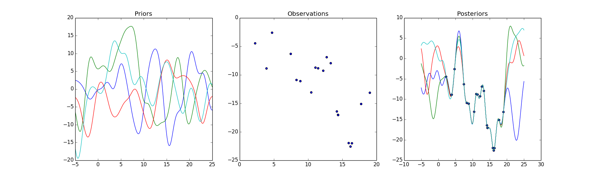
fig, axarr = plt.subplots(1, 3)
# Plot Priors
axarr[0].set_title('Priors')
for k in range(N_prior_sample):
axarr[0].plot(x_gp, y_prior[k])
# Plot the observations
axarr[1].set_title('Observations')
axarr[1].scatter(x_observation, y_observation)
# Plot the sampled functions from the Gaussian Process
axarr[2].set_title('Posteriors')
axarr[2].scatter(x_observation, y_observation)
for k in range(N_posterior_sample):
axarr[2].plot(x_gp, y_posterior[k])
plt.show()

Leave a Comment