Faster Neural Radiance Fields Inference
The Neural Radiance Fields (NeRF) proposed an interesting way to represent a 3D scene using an implicit network for high fidelity volumetric rendering. Compared with traditional methods to generate textured 3D mesh and rendering the final mesh, NeRF provides a fully differntiable way to learn geometry, texture, and material properties for specularity, which is very difficult to capture using non-differentiable traditional reconstruction methods.
Let’s first go over the rendering equation. For each ray, we compute a weighted sum (integrate) of all colors samples $\mathbf{c}_i$ from the line of sight where the weight is visibility ($T_i$) times the opaqueness ($1 - \alpha_i$) of the point. Basically, the weight is the geometric distribution of transparency $\alpha$.
\[\begin{align} \hat{\mathbf{c}} & \approx \sum_i^N T_i \alpha_i \mathbf{c}_i \\ \hat{\mathbf{c}}(\mathbf{r}) & \approx \sum_i^N \left( \prod_{j = 1}^{i - 1} (1 - \alpha(\mathbf{r}(t_j), \Delta_j)) \right) \alpha(t_i, \Delta_i) \mathbf{c}(\mathbf{r}(t_i), \mathbf{v}) \end{align}\]Note that the equation does not specify how to sample $t_i$ or the number of samples $N$ required. The number of samples and where we sample $t_i$s naturally affect the accuracy and speed of the approximation. This sounds like a sampling problem that we are familiar with in statistics.
NeRF Inference: Probabilistic Approach

The original NeRF proposed a two-stage system where the first stage implicit network generates a probability distribution on a uniform samples along a ray and the second stage uses this uniform distribution to do importance sampling along the ray for more fine-grained samples. This approach allows the network to sample more densely on regions with support or high opaqueness, but it requires the some substantial number of initial uniform samples along a ray to create somewhat accurate probability distributions. However, most of these samples 1) fall on the empty space and 2) does not affect the final color values when these samples are behind a surface (you cannot see through).
Faster Inference: Efficient Ray-Tracing + Image Decomposition
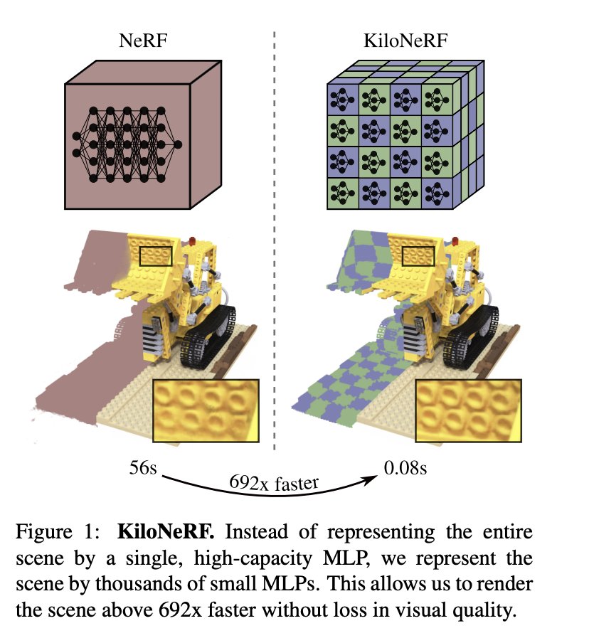
Then, if we remove redundant samples such as samples on the empty space and samples behind the surace, how much speed up can we achieve? The KiloNeRF 1 provides some insights about this question.
| Method | Render time | Speedup |
|---|---|---|
| NeRF | 56185ms | - |
| NeRF + ESS + ERT | 788ms | 71 |
This is the table 2 from the KiloNeRF paper. Empty Space Skipping (ESS) and Early Ray Termination (ERT) can drastically speed up the inference as it minimizes the number of samples. However, to use ESS, we need to know the geometry explicitly which seems to defeat the purpose of implicit networks, but I’ll get into the details later. For ERT, we can stop the ray marching when the visibility of a ray drops below a certain threshold. Both of which reduces the number of samples required for inference.
Then, how do we cache the geometry explicitly to prevent unnecesarry queries on the empty space?
Voxel Grid
The most straight forward way to cache the occupancy of a 3D space is saving it using a dense voxel grid. A dense voxel grid provides the fastest way to query a value since it only requires a ravel operation which is a series of products and sums. Given this voxel grid, we can use an efficient ray marching method 2 to skip empty voxels fast.
However, as you have guessed, dense voxel grids have cubic memory complexity which would be prohibitive to use for high resolution grids. High resolution grids can save more time as we can skip more space by representing the empty space in a fine-grained way, which would reduce the number of NeRF feed forward passes.
Sparse Voxel Grid and Octrees: Spatial Sparsity
To increase the resolution of a voxel grid, we have to harness the sparsity of 3D space. A sparse voxel grid is a sparser version of a dense grid which only saves non-zero elements. The data in this sparse voxel grid is a list of coordinates and corresponding data. To extract values from this list of coordinates and data, we have to search for whether the target point is present in this list and this can be done either with going over all the elements in this list and see if there is a hit; or we need a data structure that can accelerate querying. There are a few data structures that can accelerate search: a tree and a hash table. If we use a binary tree for search, this would be a variant of a KD tree. If we divide all 3 dimensions and have 8 leaves for each node, this becomes an octree.

Neural Sparse Voxel Fields 3 proposed learn a sparse voxel grid in a progressive manner that increases the resolution of the voxel grid at a time to not just such represent explicit geomety but also to learn the implicit features per non-empty voxel.

PlenOctree 4 also uses the octree structure to speed up the geometry queries and store the view-dependent color representation on the leaves. For the view-dependent color representation, the authors propose to use the spherical harmonics coffeficients of RGB values.

Lastly, Baking Neural Fields 5 uses a slightly different data structure to save the explicit geometry. The coarsest level consists of a $(N / B)^3$ resolution dense voxel grid that points to the blocks of a size-$B^3$ dense voxel grid. This makes use of sparsity of the 3D space while making data somewhat contiguous for efficient memory access. Also, they mention that octrees’ intermediate non-leaf nodes and tree traversals required to query can incur a significant memory and time overhead. There is an another important concept that speeds up the inference in this paper which I will discuss later.
Smaller Networks: Spatial Decomposition and Specularity Decomposition
One of the most obvious steps to do faster inference is to make a systems small and computationally less demanding. However, this is difficult to achieve without making some sacrifice on the performance. However, there are some methods that propose to make a NeRF network smaller by decomposing some properties of rendering: spatial decomposition and image decomposition.
Spatial Decomposition of NeRF
When we render a scene, surfaces that are visible to our view are rendered, but not the other occluded surfaces. So, using a large NeRF that represents the entire scene to extract the information about a small portion of the space could be inefficient. KiloNeRF 6 proposes to decompose this large deep NeRF into a set of small shallow NeRFs that capture only a small portion of the space. This allows the nerfs to be very small and shallow as the amount of information required to capture for each nerf is relatively small. However, during the rendering process, a ray has to go through a different set of NeRFs each of which take a different number of samples. This dynamic rather than static parameter loading requires a special CUDA kernel for a proper speedup.
Another spatial decomposition can be found in Neural Sparse Voxel Fields (NSVF) 3. NSVF speeds up the rendering by first approximating the geometry of an object with a coarse voxel grid for faster ray tracing, but another benefit comes from the spatial decomposition of the space itself. Each non-zero voxel or occupised voxel has a feature vector that encoded the geometry and texture of the space the voxel occupies. Compared with the NeRF that uses one monolithic MLP, NSVF uses numerous smaller features to encode the geometry. This spatial decomposition allows us to 1) scale the system and allows us to learn a large space as the parameter grows additively rather than multiplicatively 2) speed up the inference using empty space skipping or faster ray-tracing 3) allows spatial editing since the geometry is somewhat explicit.
Image Decomposition of NeRF
An image can be decomposed into 1. a view-dependent color or albedo that depends only on the global illumination and the color of the object. 2. a view dependent color or specularity that depends not just on the color of the object, but also on the directional lights as well as the view direction of a camera.

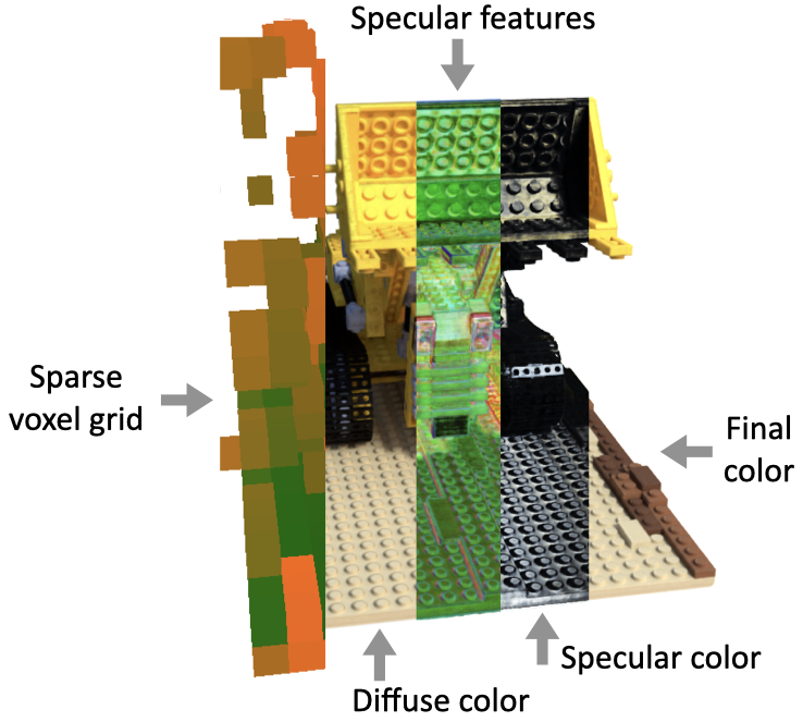
Baking Neural Radiance Fields (SNeRG for short) 5 proposes to decompose an image into the diffuse color and specularity so that the inference network handles a very simple task. This makes the network very small and shallow compared with the other NeRF networks.
The paper also uses caching the intermediate features on the sparse voxel grid. However, unlike other NeRF networks that evaluate color per 3D sample, SNeRG computes weighted sum of the intermediate features and then evaluate color per pixel, which significantly reduces the number of feed forward passes.
Analysis
There are many components for faster inference of NeRF that I summarized in this blog. Some of which are not orthogonal to each other and thus allows us to speed up further. I’ll go over these components and share my thoughts on faster inference of NeRF.
Explicit Geometry Representation
One of the most important component that is found in almost every fast NeRF inference papers is explicit geometry representation. This can be a form or a dense voxel grid, an octree, or a sparse voxel grid. All these allow the rendering process to sample points along a ray that are occupied rather than wasting computation on empty space. You might wonder why we go back to explicit geometry representations when the implicit networks were proposed to overcome limitations of discrete representations? This I think is slightly orthogonal to the direction we discussed in this blog. The NeRF and implicit networks proposed a way to learn 3D geometry in a completely differentiable manner. This differentiable learning allows us to bypass the 3D reconstruction process that involves finding 2D correspondences, 3D point cloud generation, multi-view stereo reconstruction, texture mapping, material estimation, and illumination estimation. Rather, we assign one network to handle all these steps in 3D reconstruction and generate realistic rendering in a differentiable way which allows us to extract as much information from the input and minimizes loss of quality.
Discrete vs. Continuous Representation
Regarding this explicit geometry representation, all papers use discrete voxel grids rather than a continuous point cloud or meshes. This is due to the efficiency of discrete representations. Since these representations are structured, we can make use of the structure to accelerate spatial operations. To name a few, we have faster random access, faster memory access using L1 caches, as well as faster ray traversal using voxels. Continuity is important in learning for differentiability, but as we have seen in the SNeRG 5, representing a scene using high resolution grids can make almost everything look contiuous like in 4k images.
Decomposition
Increasing the parameter space multiplicatively would probably make everything impossible to learn. That is why making some level of independence assumptions even when it is clearly not can make things faster and better. In other words, $P(X, Y) \approx P(X)P(Y)$ make things more manageable and faster. Mean-field approximation is a good example of such decomposition.
The same principle can be applied to 3D representation and graphics. Instead of representing a 3D geometry with one monolitic representation, decomposing it reduces the complexity like we saw in KiloNeRF. Similarly, SNeRG decomposed an image into view-dependent and view-independent images to reduce the complexity of the rendering network. Such decompositions allow us to model the system whose complexity increases additively rather than multiplicatively. This is the key to a scalable system.
Postscriptum
This is not a complete list of faster NeRF papers. Please feel free to recommend me more interesting papers that you think I should include on this blog post. Also, feel free to comment on errors that you find in this post and I’ll promtly fix errors.


Leave a Comment